COVID-19 Post Stay-At-Home Analysis Summary

Posted on April 22, 2020

State of Ohio Covid-19 post stay at home options impact analysis summary utilizing a transmissibility modified SEIR modeling technique.

Summary Overview

This summary discusses the findings from an Ohio focused COVID-19 modified SEIR (Susceptible, Exposed, Infected, Recovered) model that was created to correct perceived shortcomings in existing predictive models which tend to overestimate the number and rate of infections. This summary is intended for use as another data point in the ongoing quest to improve our understanding of the novel COVID-19 virus and it’s impact on Ohio’s population. This document is not formatted as or intended to be a formal white paper on the topic but I felt the findings were worth a brief summary.

Model correlation and baseline

The model correlation and baseline section discuss and summarize the thought process behind the critical model inputs and adjustments.

Transmission Rate (R0):

There are several critical inputs to modeling infectious diseases. One of the most significant being the determination of the initial level of transmissibility, R0, as it drives the ramp rate, peak infections, and herd immunity level for a given infection. Early analyses of R0 tend to overestimate the transmissibility level which could be caused by the increase in testing rate exceeding the actual transmission rate of the disease. Many curves are generated to “fit” the positive test level without complete data as to the actual transmissibility of the virus. This was seen in the early analysis of Wuhan, China, where some initial estimates of an R0 were as high as 3.1 in early publications.

After reviewing several papers on COVID-19 R0 I determined Zhang’s[1] analysis of the Diamond Princess cruise ship represented the most compelling case for the following reasons: 1) The cruise ship represented the closest example to a controlled case study; 2) Introduction and timing of the virus was determined to a high degree of confidence; 3) The level of testing during several weeks of quarantine provided a detailed look back at transmissibility leading up to ships arrival in Japan. The results of the Zhang[1] paper show the Diamond Princess had experienced an R0 of 2.28 (95% CI). Since ~3700 people on a cruise ship represents an extreme level of population density and social interactive behavior, an R0 of 2.28 was considered the most likely upper limit for COVID-19.

The next step was to determine an R0 social density and behavioral adjustment between the Diamond Princess and the State of Ohio. This was estimated by creating a model of New York City’s COVID-19 experience and fitting a curve to it and then estimating the difference between NYC and Ohio based on factors like population density and use of public transportation (societal interaction was considered neutral as greeting customs and conversational spacing are similar between the two regions). The NYC model had a best R0 curve fit of 2.15. Overall the State of Ohio has a much lower population density and 2 limited public transportation system when compared to New York City and as such Ohio’s R0 was reduced an additional 0.15 to a final value of 2.0 for this analysis.

Mean latent Period (1/σ):

The mean latent period was estimated based on several preliminary study reviews which were in general agreement around a mean value of ~5.2[2].

Mean infection Period (1/γ):

Mean infection period varied greatly between studies with most between 7 and 18 days[3],[4],[5]. The studies with the higher numbers tend to focus on the confirmed infected which usually involve lengthy periods of hospitalization. Very few addressed inclusion of the high level of asymptomatic cases (discussed later) with shorter durations. Also, the longer the infection period the flatter the curve so selecting a lower number is considered the conservative approach with respect to the peak infected value. For this analysis, a mean infection period value of 8 was chosen.

Adjustment to SEIR Modeling Theory:

A standard 4 ODE SEIR model takes into account the change over time for the susceptible, exposed, infected, and recovered aspects of the virus but does not fully address a fifth variable which is transmission rate. Figure 1 is an example of an SEIR model run with an R0 value of 2.0 for an Ohio population (N) of 11.7M residents.

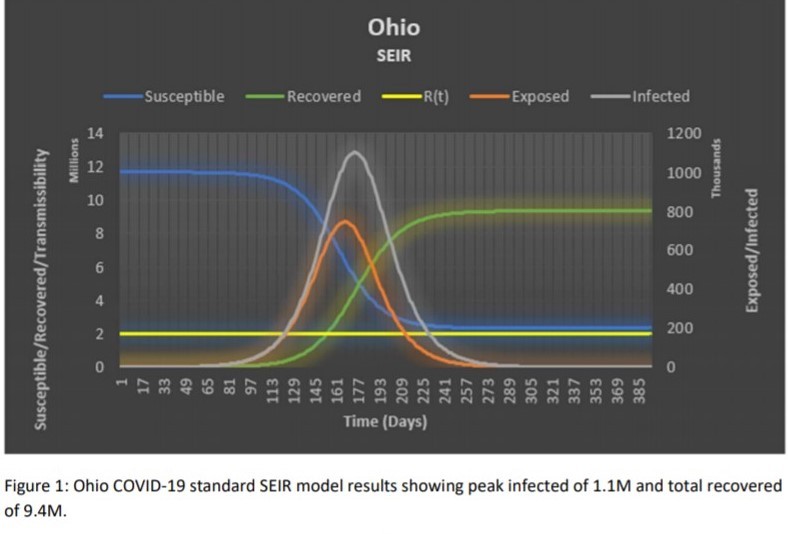
To determine confidence in the standard SEIR model, I compared it to the independent calculation of herd immunity. The theory being, if the herd immunity percentage agreed with the standard SEIR recovered percentage, it would provide confidence in the model as herd immunity is established. The herd Immunity percentage for a homogenous group impacted by a virus with an R0 = 2.0 is 50%. From the above SEIR Figure 1 the recovered percentage is ~80% which indicates the SEIR model is potentially over estimating infection rates.

A review of the SEIR equations led to the conclusion that the transmissibility variable (β) used in the Susceptible and Exposed formulas should not be fixed and should be treated as a separate time dependent variable. By incorporating this change the modified SEIR model predicted a recovered population of 5.6M or 51.6% which aligns much closer with the herd immunity calculation result (see Figure 2):

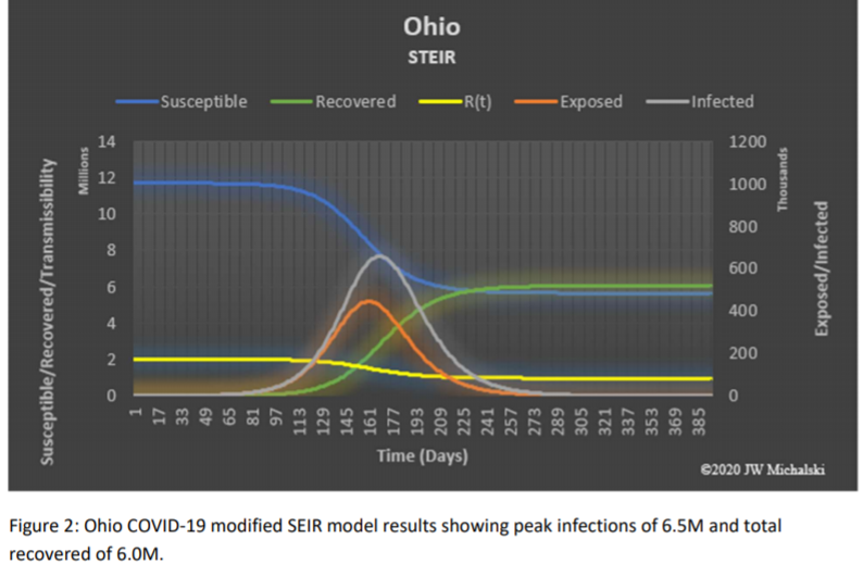
Another significant observation from the modified SEIR model is the reduction in predicted peak infected versus the basic SEIR model, 0.7M vs 1.1M respectively. This may help explain the series of significant over estimates and revisions seen in reports using the basic SEIR model as a baseline.

Lastly, the modified SEIR model contains other transmissibility adjustments to account for impact of temperature (ΔT) and humidity (ΔrH) based on Wang’s[6] study as well as other changes to over time such as the effect of social variations/directives which were not included in Graph 2 results.

State of Ohio Modified SEIR Model Forecast

Case 1: Do nothing

The first case is the “do nothing” case. This includes no closures or modifications to daily life, including no social habit modifications or distancing. However, the “do nothing” case does include a temperature/humidity shift from the results of Wang’s[6] COVID-19 temperature/humidity impact study. Columbus, Ohio weather was used as being a central point in the state. To be conservative, the temperature and humidity effects are only applied to anticipated summer indoor changes as that is where the majority of viral exposure occurs. Further transmissibility reduction could be justified by a study of summer indoor/outdoor viral exposure but was beyond the intent of this analysis to provide reasonable worse case scenarios.

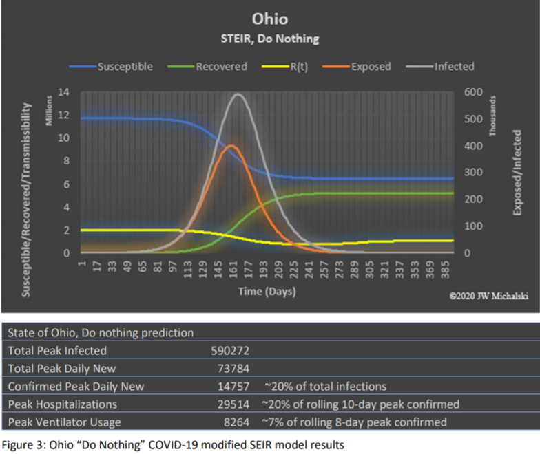
The “do nothing” results show that an unmitigated response to COVID-19 in Ohio may have overwhelmed the existing medical system[7]. The total peak values include all infections in-which 80% in this analysis are asymptomatic or mild and not confirmed based on the results of several COVID-19 studies[1],[8],[9]. The studies varying between 50% for the Diamond Princess[1] to 98% in Bendavid’s[8] Santa Clara sampling. The Diamond Princess data was discounted as the average age of the passengers was significantly higher ( ̄x=58) than Ohio ( ̄x=39) in which you would anticipate a higher percentage exhibiting symptoms. The selection of 80% was in the lower range of the other reports to remain conservative.

Case 2: Social Distancing Scenario 1

Social distancing scenario 1 implements a gradual transmissibility reduction due to social distancing and federal and state recommended restrictions until the transmissibility level goes to Rt = ~1.0, biased by the mean latency, when the Governor of Ohio implemented a “stay at home” order for 6 weeks (22- Mar-2020). The transmissibility is adjusted over Easter weekend to account for increased social interaction and then increases 1-May-2020 directly to the US Phase III economic recovery plan. The results are shown in Figure 4.

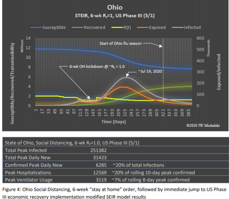
Social distancing scenario 1 shows a moderate risk in this conservative approach of nearing Ohio’s available hospital/ventilator availability. The benefit of this scenario is that the peak occurs in the summer months to reduce the potential of a major second wave occurring concurrently with the 2020/21 flu season.

Case 3: Social Distancing Scenario 2

Social distancing scenario 2 applies all the same transmissibility reduction profile as scenario 1 up to and including the “stay at home” order. After the “stay at home” order, scenario 2 increases transmissibility on 1-May-2020 to the US Phase II plan level and again on 3-Aug-2020 to US Phase III level after the peak infected rate is achieved plus 14 days. The results are shown in Figure 5.

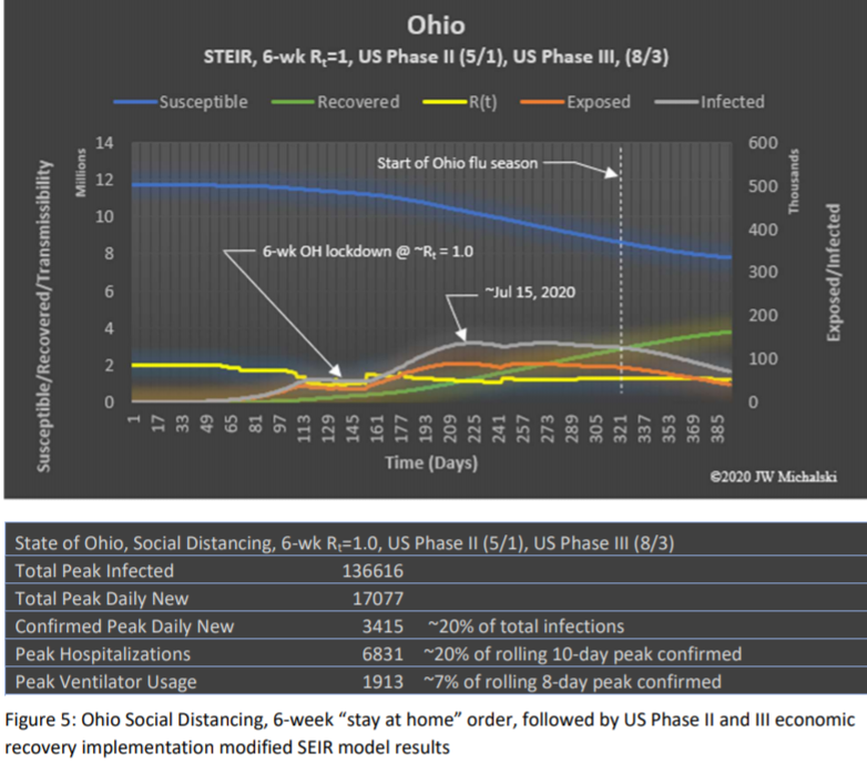
The results show additional peak reduction versus social distancing scenario 1, however there is a second peak which is slightly less than the first. To review US Phase III timing sensitivity, if the US Phase III implementation date is moved two days earlier, the model shows the second peak will be larger than the first. It is also important to note that the social distancing scenario 2 enters Fall 2020 with a significant percentage of susceptible population which could result in a large second wave if mitigations are not managed properly. Mitigation planning should be mindful of this risk and target the peak to occur as close to mid-summer as possible to maximize the natural transmissibility reduction from heat and humidity.

Case 4: Social Distancing Scenario 3

Social distancing scenario 3 applies all the same transmissibility reduction profile as scenarios 1 and 2 up to and including the “stay at home” order. After the “stay at home” order, scenario 3 increases transmissibility on 1-May-2020 to the US Phase I plan level, again on 21-July-2020 after a two-week reduction in US Phase I infected to US Phase II and finally on 17-Aug-2020 to US Phase III two weeks after the second peak is achieved. The results are shown in Figure 6.

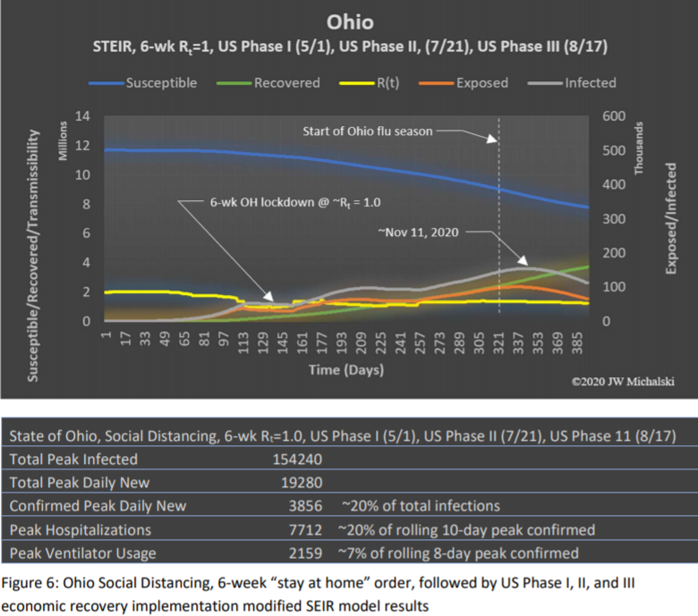
The results of social distancing scenario 3 brought to light the risk outlined in scenario 2. If US Phase I is implemented with an average transmissibility increase that is muted by the summer heat and humidity, the model shows there will be a shallow peak in mid-July. Phase II would result in another muted peak that is higher than the first. US Phase III would be implemented just prior to the school year. The increased social interaction of school being in session combined with the temperature and humidity transmissibility benefit declining results in a much larger infected peak occurring in mid-November.

Observations/Conclusions

The standard SEIR modeling techniques may be overstating infected/recovered numbers due to fixed transmissibility rates within the model. By adding a time dependent transmissibility variable to the modeling, the predicted infected/recovered population is significantly reduced and better aligns with the independently calculated herd immunity percentage.

Since the COVID-19 virus is widespread in Ohio, the focus should shift from attempting to eliminate the spread to managing the timing and peak infected while protecting the most vulnerable. Based on the modified SEIR modeling results, the State of Ohio should ease the lockdown social restrictions as soon as new guidelines for non-essential business operation can be released. The easement should be in agreement with social distancing scenario 1 or 2 so the spread of the virus can increase at a moderate rate during the summer where temperature and humidity transmissibility reductions will contribute to a manageable peak infected rate.

Results from social distancing scenario 3 show that not increasing the transmissibility rate to a point in which a significant portion of the population moves to recovered over the summer could result in a larger peak in the Fall/Winter of 2020. The impact of this would be compounded by the influenza season and both would be competing for limited hospital/PPE/medical resources. In addition, the “triple peak”, with each subsequent peak being greater than the one before, may cause societal panic or distrust in government officials to manage the crisis.

Finally, this analysis did not consider the possibility that COVID-19 has been in circulation in the United States for many months as some preliminary studies are now suggesting. If this theory establishes credibility once widespread serological antibody testing becomes available, the results herein are considered even more conservative.

References (in order of appearance):

Zhang S, Diao M, Yu W, Pei L, Lin Z, Chen D, Estimation of the reproductive number of novel coronavirus (COVID-19) and the probable outbreak size on the Diamond Princess cruise ship: A = data-driven analysis. International Journal of Infectious Disease, 22-Feb-2020
Lauer S A, K H Grantz, Q Bi, F K Jones, Q Zheng, H . Meredith, A S Azman, N G Reich, J Lessler. The Incubation Period of Coronavirus Disease 2019 (COVID-19) From Publicly Reported Confirmed Cases: Estimation and Application. Annals of Internal Medicine, 2020
Li, Q. Early transmission dynamics in Wuhan, China, of novel coronavirus–infected pneumonia. N. Engl. J. Med. 2020
Santilli M, How Long Do Novel Coronavirus Symptoms Last? Women’s Health, 31-Mar-2020
Aubry A, How Long Does It Take To Recover From COVID-19? Shots Health News from NPR, 13-Apr-2020
Wang, J, K Tang, K Feng and W Lv. High Temperature and High Humidity Reduce the Transmission of COVID-19, 9-Apr-2020 (in peer review)
Exner, R, How many hospital beds are near you? Details by Ohio county, Cleveland.com, 23-Mar-2020
Bendavid E, B Mulaney, N Sood, S Shah, E Ling, R Bromley-Dulfano, C Lai, Z Weissberg, R Saavedra Walker, JTedrow, D Tversky, A Bogan, T Kupiec, D Eichner, R Gupta, J P A Loannidis, J Bhattacharya. COVID-19 Antibody Seroprevalence in Santa Clara County, California, medRxiv, 14-Apr-2022
Saltzman J., Nearly a third of 200 blood samples taken in Chelsea show exposure to coronavirus. Boston Globe, 17-Apr-2020
Michael J. Covid-19: four fifths of cases are asymptomatic, China figures indicate. theBMJ.com. 2-= Apr-2020

News